Background
When we read a science paper to progress our understanding of a topic, it is imperative to know how to interpret the results section—you know, that section we have all casted a blind eye to before heading to the discussion!
The inability to interpret research findings appropriately is part of the reason for so much debate within the nutritional field. Or science, generally, to be honest. It is common for two people (including experts) to read the same study and reach conflicting conclusions. I have lost count of the number of times people have sent me ‘supporting evidence’ for a claim when the results indicate otherwise upon inspection. Why? Numerous factors. More often than not, however, it is because one party does not have a basic understanding of statistics.
For this reason, this article provides a basic overview of inferential statistics—that is, the collection of tools and techniques to make inferences from data. Specifically, I want to touch on three statistical results that everyone needs to be mindful of when analysing the results section of any study: p-values, point estimates, and confidence intervals.
P Values
Let’s start with p-values—this is probably the statistical measure that you are most familiar with. It is commonplace to read a study and head straight for that p-value.
Was the result statistically significant (p ≤ 0.05) or was it not (p > 0.05)? Many people think they have found something interesting if the result is the former; if not, it is nothing to care about. Dare I say this interpretation was as much as my (lack of) statistical brain would comprehend throughout my university years. My attention-deficit disorder brain wanted the study to just tell me the result, it’s importance, and be on its merry way. Rarely, if ever, would it question the p-value or try to comprehend its influence on my interpretation of the results, or the broader research area. This was my own wrongdoing, though, as it turns out the p-value is the most frequently misinterpreted statistical measure. By far.
To better understand the p-value, let’s clarify why it was implemented in scientific research. What was its purpose? I’m sure statisticians could enter into a long rant here, but I’ll try to keep it brief.
The p-value was introduced to complement the Theory of Probability, stating that “variation must be taken as random until there is positive evidence to the contrary”. In other words, if you find an association within a data set, you assume it is random until a statistical test measures the compatibility with this assumption.
Introducing the p-value. A simple way to think about the p-value is that it summarises the compatibility between data and a pre-defined hypothesis (also called a ‘test hypothesis’). The test hypothesis is always specific to the study you are reading, but most often it is a ‘null’ hypothesis. This postulates the absence of an effect; even if there is an association, the null hypothesis assumes it is random.
What do I mean by the term ‘compatibility’? Well, the definition of a p-value revolves around probabilities. A little bit more detail is required, though. To quote the American Statistical Association (ASA) 2016 statement [1], “…a p-value is the probability under a specified statistical model that a statistical summary of the data (e.g., the sample mean difference between groups) would be equal to or more extreme than its observed value”. Yes, quite a mouthful. Confusing, too.
The “would be” part is particularly confusing—would be if what?. Let’s reframe this for clarity. Another way to state the definition of a p-value is… given repeated sampling in the same population, the p-value is the probability that chance alone would lead to a difference between groups as large as observed in the study. I know that even my rejigged definition still requires a few reads to grasp. Still, I hope that it at least clarifies the p-value is comparing what was observed to what we expect to observe when there is no true effect.
And because we are discussing probabilities here, we should know that the p-value is measured on a scale between 0 to 1. This scale is what summarises the compatibility of the data with the null hypothesis:
- 1 on the scale (p = 1.00) means that the data is fully compatible with the null hypothesis.
- 0 on the scale (p = 0.00) means that the data is fully incompatible with the null hypothesis.
However, certainty and impossibility are incomprehensible extremes of probability and, in reality, no study will ever find that p = 0 or p = 1. Rather, the p-value will always sit somewhere between these two extremes. The lower the p-value (closer to p = 0.00), the less compatible the data is with the null hypothesis; the higher the p-value (closer to 1.00), the more compatible the data is with the null hypothesis. In turn, despite the fact that no p-value inherently reveals the plausibility or truth of an association or effect, lower p-values may be used as contributing evidence against the null hypothesis of no association or difference or effect. This “contributing evidence” is not because small p-values are rarely observed given the null hypothesis is true (a common misinterpretation), but actually because they are relatively less likely to be observed when the null hypothesis is true compared to an alternative hypothesis.
Understanding the prior is key to knowing why many people’s interpretation of a p-value is faulty. Typically—and I was not an exception—people think that p ≤ 0.05 is a demonstration of a “true effect” and p > 0.05 is a demonstration of “no effect”. Clearly, we have already established why this is fundamentally incorrect by knowing what the p-value actually measures. It does not measure an effect; it measures the statistical compatibility with no effect. This begs the question, then, why is the cut off for what is known as “statistical significance” set at p ≤ 0.05? (at least in health sciences). I pondered this question for a while, but it turned out that there was no logical answer. The 0.05 cutoff for statistical significance, known as the ‘alpha level’ of the test, is used because researchers in the field largely agree upon it and apply it consistently to help reach conclusions. There is nothing special about this specific number, though. The fact remains that no p-value inherently reveals the plausibility or truth of an association or effect and therefore and, as per the probability continuum, statistically nonsignificant p-values (p > 0.05) do not necessarily contradict statistically significant p-values (p ≤ 0.05) just because they lie on opposite sides of a statistical fence. The same 2016 ASA statement that I cited earlier clarified that statistical significance testing and p-values never substitute for scientific reasoning [1]. The p-value simply is what it is; to be interpreted as a continuous variable and not in a dichotomous way.
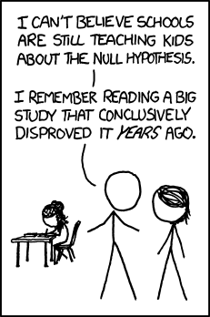
This being said, the nature of the test’s alpha level, and statistical significance in general, should not imply that they have no utility. Tunc et al. [2] argue that “the function of dichotomous claims in science is not primarily a statistical one, but an epistemological and pragmatic one. From a philosophical perspective rooted in methodological falsificationism, dichotomous claims are the outcome of methodological decision procedures that allow scientists to arrive at empirical statements that connect data to phenomena.” At the end of the day, there has to be some kind of distinguishing element between evidence that is used for or against a real-world decision; we require some framework for epistemological consistency. This does not mean that we should leave our hands tied based on this probability alone, but p-values and statistical significance testing can be part of a holistic approach to study interpretation and decision-making. We can use p-values to infer what the data indicate about the effect and interval estimates concerning the null hypothesis. Thus, we should always use our wider knowledge of research design and other statistical measures to reach overall conclusions about what the data infer about a specific research question. This same narrative is highlighted superbly in a recent paper titled ‘There is life beyond the statistical significant’, where Ciapponi et al. [2] state that, “…rather than adopting rigid rules for presenting and interpreting continuous P-values, we need a case by case thoughtful interpretation considering other factors such as certainty of the evidence, plausibility of mechanism, study design, data quality, and costs-benefits that determine what effects are clinically or scientifically important”.
So there we have it, p-values. Pretty complex, right? I hope to have highlighted some correct interpretations that maybe you were unaware of. Maybe you were already well aware and this is a nice reminder. In any case, I leave this section with five more correct interpretations of a p-value that I believe are not currently well-appreciated in nutrition science discussions:
- If two groups are “not significantly different”, this does not mean “not different from”. Commentary on “no differences” between groups based on statistical nonsignificance is erroneous and misleading. It only takes a brief look at data to see differences (even if simply explained by randomness) that contributed to a p-value below 1.
- The p-value is not the probability that chance produced an association, i.e. if p = 0.25, this does not mean there is a 25% probability that chance produced the association. A couple of reasons explain why this is wrong. First, the statistical significance test already assumes that chance is operating alone. Second, the p-value refers not only to what we observed but also to observations more extreme than what we observed.
- A statistical significance test is not “null” if p > 0.05. A p-value should never be used to affirm the null. The null hypothesis is assumed to be true in the calculation of the p-value.
- A large p-value is not necessarily evidence favouring the null hypothesis’ truthfulness. A large p-value might indicate that the null hypothesis is greatly compatible with the data, but by definition, any p-value below 1 implies that the null hypothesis is not the most compatible hypothesis with the data.
- The p-value itself is simply an estimation and one that is computed from its own assumptions. Not only do we have to assume that the statistical model used to compute the p-value is correct, but also that there is no form of bias (confounding, information, and selection bias) distorting the data in relation to the null hypothesis. The latter, in particular, is often a very strong assumption.
Point Estimate and Effect Size
To balance out the complexities of the p-value, we will now move to effect sizes which are relatively easier to comprehend yet still contain valuable information. In statistical inference, an effect size is the magnitude of the outcome difference between study groups. This statistical measure belongs within the category of what are known as ‘point estimates’—these terms tend to be used interchangeably without issue.
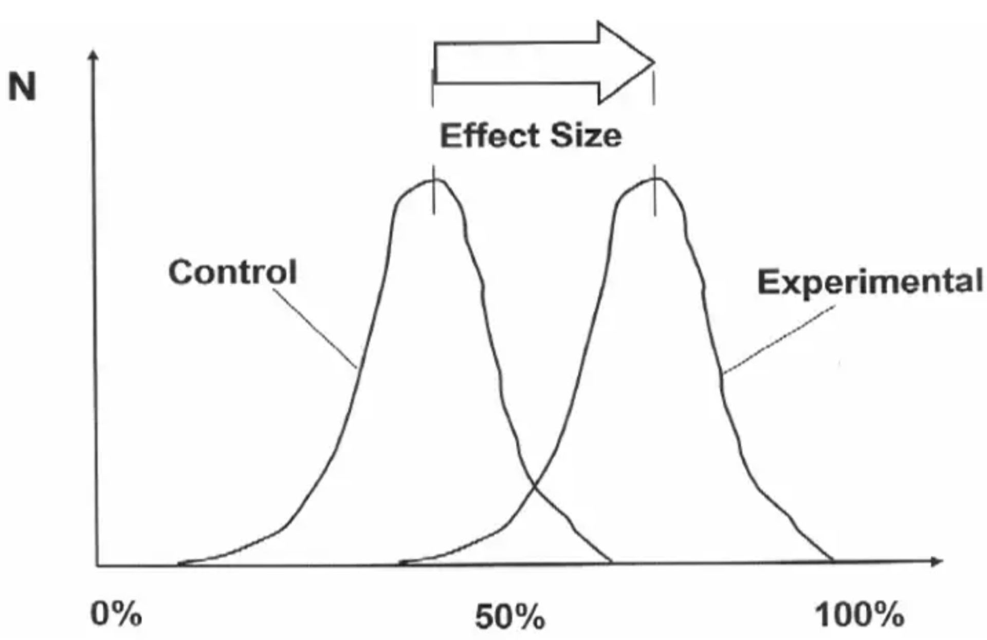
The “effect” is then attributed to some difference in exposure between study groups, such as the difference in the consumption of a certain food or nutrient. If we take a nutrition-specific example, an effect size of interest could be the difference in cardiovascular events between two groups with varying exposure to saturated fat consumption. Usually, this difference will be reported in relative terms such as a decimal or percentage difference of one group compared to another—check the methods section of a study to know the specifics! But whatever the effect size is reported as, the reader is always being given some sort of information about the magnitude of a statistical difference. Quite important! In the study results section, you will often see the effect size written as-is below (taken from Hooper et al. [3]).

In this example, the effect size is reported as a “21% reduction in cardiovascular events in people who had reduced SFA compared with those on higher SFA”. So in this sentence alone, the researchers are telling you the magnitude of difference (a 21% reduction) between specific groups (exposed to different intakes of saturated fat) with respect to a specific outcome (cardiovascular events). You will usually see the group difference reported in both decimal and percentage terms—but remember that a 21% effect size is not reported as 0.21; it is reported as 0.79, which is a 0.21 difference from 1.00 (with 1.00 always representing the control or comparison group). And although I said point estimate and effect size tend to be used interchangeably, know that people usually refer to the point estimate in reference to decimal terms (0.79) and the effect size in percentage terms (21%).
The effect size is just how it sounds, then. Effect sizes estimate the ‘size’ of an ‘effect’ with some measure of magnitude. No surprises. But why is this additional information about effect size important? Can you not just use the p-value? Well, no. The p-value covered previously does not reveal the size of an effect, only the compatibility of the data with no effect, and there are many benefits to knowing the effect size. The obvious benefit is the effect sizes practical value for nutrition practitioners. As a nutrition practitioner myself, I might use the effect size to manage client expectations about how much difference is expected from a certain dietary intervention. For example, should we tell clients that increasing their protein intake by 50% might result in dramatic muscle mass changes or only small changes? Is the magnitude of benefit worth it? The estimated effect sizes from research can guide us here.
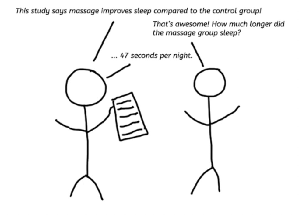
However, a less obvious benefit to knowing the effect size is actually when trying to decipher whether a true effect exists at all. Because although there is no reason to suspect large true effects are more prevalent than small true effects, we must acknowledge that we can only infer true effects via the scientific method, and there are many research biases (confounding, information, and selection bias) that interfere with making reliable estimations. Therefore, we might say that all else held equal, we are more confident inferring true effects from larger estimated effects; there is less chance that some known or unknown biases are fully responsible for the estimated effect if it is larger. For example, all else held equal, we will probably be more confident in an effect when a dietary exposure hypothetically increases the prevalence of a disease by 1000% compared to 1%. Arguing otherwise would appear to indicate ignorance of scientific uncertainties. I would suggest reading an interesting paper by Michael Hofler [3] for more thoughts on this, as he also states that “…the benefit of the consideration on strength was that strong associations could not be solely due to small biases, whether through modest confounding or other sources of bias.” Keep in mind, though, that the “all else held equal” part of my statement is critical for it to remain in the appropriate context. I am not saying that we should necessarily put more faith in larger effects than smaller effects without considering other factors such as research design, p-values, and confidence intervals. Effect sizes are only one part of the puzzle. I’m sure that we will all agree that if a meta-analysis of randomised controlled trials finds a small difference between groups with narrow confidence intervals, we will be more confident this indicates a true effect than a cross-sectional study that finds a large difference between groups with wide confidence intervals. Our confidence in a true effect is based on many factors other than its estimated size.
Perhaps more importantly than these other factors, though, is acknowledging that effect sizes are inversely correlated to baseline prevalence rates. Although it can be argued that nutrition generally deals with small effect sizes (especially compared to medicine), one of the reasons for this is because dietary relationships are often focused on outcomes with high baseline prevalences (e.g., cardiovascular disease) and, as a result, there is limited scope for large effects to exist regardless of the truthfulness of the dietary relationship. So despite many strange outcries to scrap nutrition science as being able to infer causal effects because the estimated effect sizes are generally small, I don’t see why this should be the case. Differences in effect sizes do not necessarily translate to differences in importance. A dietary exposure that increases the relative risk of cardiovascular mortality by 10% can relate to the same number of deaths as another exposure that increases lung cancer mortality by 200% – should we only believe in the lung cancer risk simply because the baseline prevalence rate is lower? This would be an unwise and dangerous position to take, in my opinion. Not only could it lead to millions of unnecessary deaths, but it would mean taking a stand against discussions of causality simply due to certain study population characteristics and/or prevalences of other causes. How can this be reasonably justified? It cannot. The alternative would be to emphasise the need for nutrition researchers to appreciate the intricate complexities of research methodology and other statistical measures, hence why I am writing this article. This way, we avoid being intellectually lazy and trying to use small effect sizes as an excuse to dismiss important causal relationships as mere associations or chance findings.

Confidence Intervals
Now that we have covered p-values and effect sizes, let’s move to another extremely important result from statistical tests: confidence intervals (abbreviated as ‘CI’). If you look at a results section, the CI figure follows a calculated point estimate (the effect size in decimal terms). In fact, the point estimate will always lie within the CI—usually right in the middle if a normal distribution is assumed. For example, using the previous Hooper et al. example, we see a point estimate of ‘0.79’ (representing a 21% increase in relative risk) followed by a CI stated as ‘95% CI 0.66 to 0.93’. But what does this mean?

Unfortunately, the CI is a little complicated to understand at first, but please bear with me. The CI results from a statistical procedure that, over infinite repeated sampling and in the absence of bias, provides us with intervals containing the true value a fixed proportion of the time. And unless you are a statistical whizz already, this definition should not make much sense until we dig a bit deeper, so let’s now look at what the ‘95% CI’ part means. If we go back to p-values and remember that the alpha level of the test is almost always 0.05, we can instantly see where the ‘95% CI’ comes from. In simple math, 1 minus the alpha level (0.05) gives you 0.95 in decimal terms, and thus the ‘95% CI’ in percentage terms. This percentage is known as the ‘confidence level’ of the statistical model, which relates directly to our CI definition’s “fixed proportion of the time” aspect. Actually, if we replace this part of the CI definition with the confidence level, we get this… over infinite repeated sampling and in the absence of bias, a CI will contain the true value with a frequency of the confidence level (95%). This might make a bit more sense? I hope so. If not, let’s go further and discuss the intervals themselves. As with any interval, we must have a lower and upper bound defining the interval—in the Hooper et al. example, the lower bound is 0.66 and the upper bound is 0.93. Thus, we can say that… over infinite repeated sampling and in the absence of bias, the estimated lower and upper bounds would contain the true value with a frequency of the confidence level (95%). We could, in theory, have a 100% confidence interval; however, in reality, it would not be beneficial for capturing a confined range of numbers as the lower and upper bounds would go from negative infinity to positive infinity.

Also, keep in mind that for any single study, we cannot know if the estimated 95% CI is even among the 95% that includes the true value, or among the 5% that do not. Therefore, we cannot claim to be “95% confident” that the true value lies within the interval for any given study. This is a common misinterpretation that I hear in nutrition science discussions. Granted, this may be perceived as an extremely picky and meaningless criticism—as with most statistical debates—but we should acknowledge that the interval itself is only an estimate and one that again relies on a correct statistical model and the often strong assumption of no bias. So while the point estimate is a single number that indicates the best estimate, interval estimates provide more information about the true value we are interested in by providing us with an estimated range of values. This makes the CI a more useful statistic measure than point estimates alone. In fact, looking solely at the point estimate alone can be deceiving. For example, if a point estimate was 1.2 (let’s say indicating a 20% increase in relative risk) yet the 95% CI was 0.2 – 2.2, we probably should not make strong claims about our confidence in the estimated effect size given the wide CI’s. In this example, the confidence interval includes as much as 20% association in one direction to a 220% association in another direction. Quite a difference!

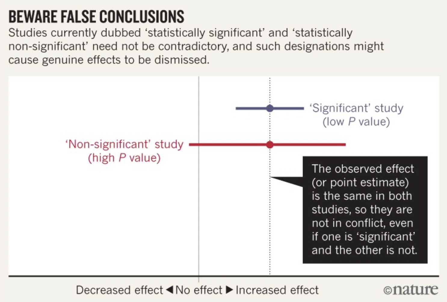
Additionally, given the direct relationship between the confidence level and the alpha level (used in statistical significance testing), it is not surprising to know that the CI directly relates to statistical significance, too. Specifically, if the CI does not contain the expected point estimate given the null hypothesis (1.00; no effect) then we have a “statistically significant” finding (p ≤ 0.05); if the confidence interval does contain the expected point estimate given the null hypothesis (1.00; no effect) then we have a “statistically nonsignificant” finding (p > 0.05). This is not all. From what we know about CI’s, we know they go beyond telling us whether the data is statistically compatible with the null hypothesis; interval estimation tells us the compatibility of the data with an alternate hypothesis. For example, if we have a 95% CI of 0.99 – 9.54, although the data is statistically compatible with the null hypothesis and “statistically nonsignificant” (the interval includes 1.00), the CI’s indicate the data is even more compatible with an association related to an alternate hypothesis. Thus, CI’s can include potentially important benefits or harms of an association not indicated by the p-value alone. In fact, if we take two p-values assessing the same relationship, one statistically significant and another statistically nonsignificant, we should not be quick to run to the conclusion that the results oppose each other. CI’s help us to understand that statistically nonsignificant results of one study do not necessarily contradict statistically significant results—I have included a forest plot below to illustrate this better. Appreciating these statistical intricacies greatly helps counter people who say that “there is research to support both sides of the argument and therefore we cannot be sure of anything.” Possibly true in some instances, but even just a quick look at CI’s can unveil a whole other truth (or estimation of the truth anyway!).
Final Thoughts
I hope to have highlighted some of the unique features of each statistical measure and why each of them is important when interpreting study results. First, we had the p-value indicating the degree to which the data is compatible with the null hypothesis that no relationship is present; however, we know that p-values alone provide limited information about data, are often misinterpreted, and do not provide information about hypotheses other than the null. Second, we had the effect size indicating the strength of an association; however, we know this is only the best estimate of the truth and is subject to variability from measurement error, various biases, and random error. Then, thirdly, we had the CI, which estimates the degree of precision characterising the point estimate and to what degree it is subject to variability. If we understand all three statistical measures together, we are putting ourselves in good stead to interpret research appropriately.
If you have enjoyed this article and want to support My Nutrition Science, please consider donating to us via this link and subscribing to our email list below.


